Normal distribution
| Probability density function The red line is the standard normal distribution |
|
| Cumulative distribution function Colors match the image above |
|
| Notation |  |
|---|---|
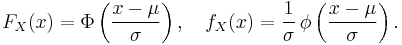
| Parameters | μ ∈ R — mean (location) σ2 > 0 — variance (squared scale) |
| Support | x ∈ R |
 |
|
| CDF | ![\frac12\left[1 %2B \operatorname{erf}\left( \frac{x-\mu}{\sqrt{2\sigma^2}}\right)\right]](/2012-wikipedia_en_all_nopic_01_2012/I/34e4c34c38cf1ce336be7623a51bc6ff.png) |
| Mean | μ |
| Median | μ |
| Mode | μ |
| Variance | σ2 |
| Skewness | 0 |
| Ex. kurtosis | 0 |
| Entropy |  |
| MGF |  |
| CF |  |
| Fisher information | 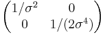 |
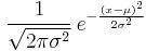
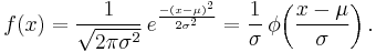
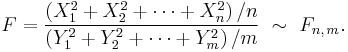
In probability theory, the normal (or Gaussian) distribution is a continuous probability distribution that has a bell-shaped probability density function, known as the Gaussian function or informally the bell curve:[nb 1]
where parameter μ is the mean or expectation (location of the peak) and σ 2 is the variance, the mean of the squared deviation, (a "measure" of the width of the distribution). σ is the standard deviation. The distribution with μ = 0 and σ 2 = 1 is called the standard normal. A normal distribution is often used as a first approximation to describe real-valued random variables that cluster around a single mean value.
The normal distribution is considered the most prominent probability distribution in statistics. There are several reasons for this:[1] First, the normal distribution is very tractable analytically, that is, a large number of results involving this distribution can be derived in explicit form. Second, the normal distribution arises as the outcome of the central limit theorem, which states that under mild conditions the sum of a large number of random variables is distributed approximately normally. Finally, the "bell" shape of the normal distribution makes it a convenient choice for modelling a large variety of random variables encountered in practice.
For this reason, the normal distribution is commonly encountered in practice, and is used throughout statistics, natural sciences, and social sciences[2] as a simple model for complex phenomena. For example, the observational error in an experiment is usually assumed to follow a normal distribution, and the propagation of uncertainty is computed using this assumption. Note that a normally-distributed variable has a symmetric distribution about its mean. Quantities that grow exponentially, such as prices, incomes or populations, are often skewed to the right, and hence may be better described by other distributions, such as the log-normal distribution or Pareto distribution. In addition, the probability of seeing a normally-distributed value that is far (i.e. more than a few standard deviations) from the mean drops off extremely rapidly. As a result, statistical inference using a normal distribution is not robust to the presence of outliers (data that is unexpectedly far from the mean, due to exceptional circumstances, observational error, etc.). When outliers are expected, data may be better described using a heavy-tailed distribution such as the Student's t-distribution.
From a technical perspective, alternative characterizations are possible, for example:
- The normal distribution is the only absolutely continuous distribution all of whose cumulants beyond the first two (i.e. other than the mean and variance) are zero.
- For a given mean and variance, the corresponding normal distribution is the continuous distribution with the maximum entropy.[3][4]
Contents |
Definition
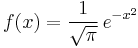
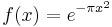
The simplest case of a normal distribution is known as the standard normal distribution, described by the probability density function
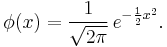
The factor  in this expression ensures that the total area under the curve ϕ(x) is equal to one,[proof] and 12 in the exponent makes the "width" of the curve (measured as half the distance between the inflection points) also equal to one. It is traditional in statistics to denote this function with the Greek letter ϕ (phi), whereas density functions for all other distributions are usually denoted with letters f or p.[5] The alternative glyph φ is also used quite often, however within this article "φ" is reserved to denote characteristic functions.
More generally, a normal distribution results from exponentiating a quadratic function (just as an exponential distribution results from exponentiating a linear function):
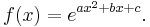
This yields the classic "bell curve" shape, provided that a < 0 so that the quadratic function is concave. f(x) > 0 everywhere. One can adjust a to control the "width" of the bell, then adjust b to move the central peak of the bell along the x-axis, and finally adjust c to control the "height" of the bell. For f(x) to be a true probability density function over R, one must choose c such that  (which is only possible when a < 0).
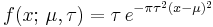
Rather than using a, b, and c, it is far more common to describe a normal distribution by its mean μ = − b2a and variance σ2 = − 12a. Changing to these new parameters allows one to rewrite the probability density function in a convenient standard form,
For a standard normal distribution, μ = 0 and σ2 = 1. The last part of the equation above shows that any other normal distribution can be regarded as a version of the standard normal distribution that has been stretched horizontally by a factor σ and then translated rightward by a distance μ. Thus, μ specifies the position of the bell curve's central peak, and σ specifies the "width" of the bell curve.
The parameter μ is at the same time the mean, the median and the mode of the normal distribution. The parameter σ2 is called the variance; as for any random variable, it describes how concentrated the distribution is around its mean. The square root of σ2 is called the standard deviation and is the width of the density function.
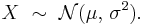
The normal distribution is usually denoted by N(μ, σ2).[6] Commonly the letter N is written in calligraphic font (typed as \mathcal{N} in LaTeX). Thus when a random variable X is distributed normally with mean μ and variance σ2, we write
Alternative formulations
Some authors advocate using the precision instead of the variance, and variously define it as τ = σ−2 or τ = σ−1.[7] This parametrization has an advantage in numerical applications where σ2 is very close to zero and is more convenient to work with in analysis as τ is a natural parameter of the normal distribution. Another advantage of using this parametrization is in the study of conditional distributions in multivariate normal case.
The question which normal distribution should be called the "standard" one is also answered differently by various authors. Starting from the works of Gauss the standard normal was considered to be the one with variance σ2 = 12 :
Stigler (1982) goes even further and insists the standard normal to be with the variance σ2 = 12π :
According to the author, this formulation is advantageous because of a much simpler and easier-to-remember formula, the fact that the pdf has unit height at zero, and simple approximate formulas for the quantiles of the distribution. In Stigler's formulation the density of a normal N(μ, τ) with mean μ and precision τ will be equal to
Characterization
In the previous section the normal distribution was defined by specifying its probability density function. However there are other ways to characterize a probability distribution. They include: the cumulative distribution function, the moments, the cumulants, the characteristic function, the moment-generating function, etc.
Probability density function
The probability density function (pdf) of a random variable describes the relative frequencies of different values for that random variable. The pdf of the normal distribution is given by the formula explained in detail in the previous section:

This is a proper function only when the variance σ2 is not equal to zero. In that case this is a continuous smooth function, defined on the entire real line, and which is called the "Gaussian function".
Properties:
- Function f(x) is unimodal and symmetric around the point x = μ, which is at the same time the mode, the median and the mean of the distribution.[8]
- The inflection points of the curve occur one standard deviation away from the mean (i.e., at x = μ − σ and x = μ + σ).[8]
- Function f(x) is log-concave.[8]
- The standard normal density ϕ(x) is an eigenfunction of the Fourier transform.
- The function is supersmooth of order 2, implying that it is infinitely differentiable.[9]
- The first derivative of ϕ(x) is ϕ′(x) = −x·ϕ(x); the second derivative is ϕ′′(x) = (x2 − 1)ϕ(x). More generally, the n-th derivative is given by ϕ(n)(x) = (−1)nHn(x)ϕ(x), where Hn is the Hermite polynomial of order n.[10]
When σ2 = 0, the density function doesn't exist. However a generalized function that defines a measure on the real line, and it can be used to calculate, for example, expected value is
where δ(x) is the Dirac delta function which is equal to infinity at x = μ and is zero elsewhere.
Cumulative distribution function
The cumulative distribution function (CDF) describes probability of a random variable falling in the interval (−∞, x].
The CDF of the standard normal distribution is denoted with the capital Greek letter Φ (phi), and can be computed as an integral of the probability density function:
![\Phi(x) = \frac{1}{\sqrt{2\pi}} \int_{-\infty}^x e^{-t^2/2} \, dt
= \frac12\left[\, 1 %2B \operatorname{erf}\left(\frac{x}{\sqrt{2}}\right)\,\right],\quad x\in\mathbb{R}.](/2012-wikipedia_en_all_nopic_01_2012/I/4cabbdc85847fa041d1240fe21633f11.png)
This integral cannot be expressed in terms of elementary functions, so is simply called the error function, or erf, a special function. Numerical methods for calculation of the standard normal CDF are discussed below. For a generic normal random variable with mean μ and variance σ2 > 0 the CDF will be equal to
![F(x;\,\mu,\sigma^2)
= \Phi\left(\frac{x-\mu}{\sigma}\right)
= \frac12\left[\, 1 %2B \operatorname{erf}\left(\frac{x-\mu}{\sigma\sqrt{2}}\right)\,\right],\quad x\in\mathbb{R}.](/2012-wikipedia_en_all_nopic_01_2012/I/111170e043276f060824cbe63b0e724d.png)
The complement of the standard normal CDF, Q(x) = 1 − Φ(x), is referred to as the Q-function, especially in engineering texts.[11][12] This represents the tail probability of the Gaussian distribution, that is the probability that a standard normal random variable X is greater than the number x. Other definitions of the Q-function, all of which are simple transformations of Φ, are also used occasionally.[13]
Properties:
- The standard normal CDF is 2-fold rotationally symmetric around point (0, ½): Φ(−x) = 1 − Φ(x).
- The derivative of Φ(x) is equal to the standard normal pdf ϕ(x): Φ′(x) = ϕ(x).
- The antiderivative of Φ(x) is: ∫ Φ(x) dx = x Φ(x) + ϕ(x).
For a normal distribution with zero variance, the CDF is the Heaviside step function (with H(0) = 1 convention):
Quantile function
The inverse of the standard normal CDF, called the quantile function or probit function, is expressed in terms of the inverse error function:

Quantiles of the standard normal distribution are commonly denoted as zp. The quantile zp represents such a value that a standard normal random variable X has the probability of exactly p to fall inside the (−∞, zp] interval. The quantiles are used in hypothesis testing, construction of confidence intervals and Q-Q plots. The most "famous" normal quantile is 1.96 = z0.975. A standard normal random variable is greater than 1.96 in absolute value in 5% of cases.
For a normal random variable with mean μ and variance σ2, the quantile function is

Characteristic function and moment generating function
The characteristic function φX(t) of a random variable X is defined as the expected value of eitX, where i is the imaginary unit, and t ∈ R is the argument of the characteristic function. Thus the characteristic function is the Fourier transform of the density ϕ(x). For a normally distributed X with mean μ and variance σ2, the characteristic function is [14]
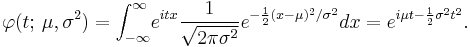
The characteristic function can be analytically extended to the entire complex plane: one defines φ(z) = eiμz − 12σ2z2 for all z ∈ C.[15]
The moment generating function is defined as the expected value of etX. For a normal distribution, the moment generating function exists and is equal to
![M(t;\, \mu,\sigma^2) = \operatorname{E}[e^{tX}] = \varphi(-it;\, \mu,\sigma^2) = e^{ \mu t %2B \frac12 \sigma^2 t^2 }.](/2012-wikipedia_en_all_nopic_01_2012/I/b26b75c799d5bde5f3429eb28db066c2.png)
The cumulant generating function is the logarithm of the moment generating function:
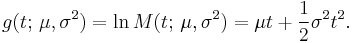
Since this is a quadratic polynomial in t, only the first two cumulants are nonzero.
Moments
The normal distribution has moments of all orders. That is, for a normally distributed X with mean μ and variance σ 2, the expectation E[|X|p] exists and is finite for all p such that Re[p] > −1. Usually we are interested only in moments of integer orders: p = 1, 2, 3, ….
- Central moments are the moments of X around its mean μ. Thus, a central moment of order p is the expected value of (X − μ) p. Using standardization of normal random variables, this expectation will be equal to σ p · E[Zp], where Z is standard normal.
- Central absolute moments are the moments of |X − μ|. They coincide with regular moments for all even orders, but are nonzero for all odd p's.
- Raw moments and raw absolute moments are the moments of X and |X| respectively. The formulas for these moments are much more complicated, and are given in terms of confluent hypergeometric functions 1F1 and U.
- First two cumulants are equal to μ and σ 2 respectively, whereas all higher-order cumulants are equal to zero.
![\mathrm{E}\left[(X-\mu)^p\right] =
\begin{cases}
0 & \text{if }p\text{ is odd,} \\
\sigma^p\,(p-1)!! & \text{if }p\text{ is even.}
\end{cases}](/2012-wikipedia_en_all_nopic_01_2012/I/79ee7c2bbdca2da8931d51e2b2eca492.png)
![\operatorname{E}\left[|X-\mu|^p\right] =
\sigma^p(p-1)!! \cdot \left.\begin{cases}
\sqrt{2/\pi} & \text{if }p\text{ is odd}, \\
1 & \text{if }p\text{ is even},
\end{cases}\right\}
= \sigma^p \cdot \frac{2^{\frac{p}{2}}\Gamma\left(\frac{p%2B1}{2}\right)}{\sqrt{\pi}}](/2012-wikipedia_en_all_nopic_01_2012/I/68bb8492fd421428882af6a3ee74a438.png)
![\begin{align}
& \operatorname{E} \left[ X^p \right] =
\sigma^p \cdot (-i\sqrt{2}\sgn\mu)^p \;
U\left( {-\frac{1}{2}p},\, \frac{1}{2},\, -\frac{1}{2}(\mu/\sigma)^2 \right), \\
& \operatorname{E} \left[ |X|^p \right] =
\sigma^p \cdot 2^{\frac p 2} \frac {\Gamma\left(\frac{1%2Bp}{2}\right)}{\sqrt\pi}\;
_1F_1\left( {-\frac{1}{2}p},\, \frac{1}{2},\, -\frac{1}{2}(\mu/\sigma)^2 \right). \\
\end{align}](/2012-wikipedia_en_all_nopic_01_2012/I/15d2a58f7cec0fb6c030622810743ef2.png)
| Order | Raw moment | Central moment | Cumulant |
|---|---|---|---|
| 1 | μ | 0 | μ |
| 2 | μ2 + σ2 | σ 2 | σ 2 |
| 3 | μ3 + 3μσ2 | 0 | 0 |
| 4 | μ4 + 6μ2σ2 + 3σ4 | 3σ 4 | 0 |
| 5 | μ5 + 10μ3σ2 + 15μσ4 | 0 | 0 |
| 6 | μ6 + 15μ4σ2 + 45μ2σ4 + 15σ6 | 15σ 6 | 0 |
| 7 | μ7 + 21μ5σ2 + 105μ3σ4 + 105μσ6 | 0 | 0 |
| 8 | μ8 + 28μ6σ2 + 210μ4σ4 + 420μ2σ6 + 105σ8 | 105σ 8 | 0 |
Properties
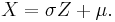
Standardizing normal random variables
As a consequence of property 1, it is possible to relate all normal random variables to the standard normal. For example if X is normal with mean μ and variance σ2, then
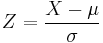
has mean zero and unit variance, that is Z has the standard normal distribution. Conversely, having a standard normal random variable Z we can always construct another normal random variable with specific mean μ and variance σ2:
This "standardizing" transformation is convenient as it allows one to compute the PDF and especially the CDF of a normal distribution having the table of PDF and CDF values for the standard normal. They will be related via
Standard deviation and confidence intervals
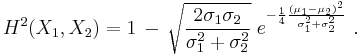
About 68% of values drawn from a normal distribution are within one standard deviation σ away from the mean; about 95% of the values lie within two standard deviations; and about 99.7% are within three standard deviations. This fact is known as the 68-95-99.7 rule, or the empirical rule, or the 3-sigma rule. To be more precise, the area under the bell curve between μ − nσ and μ + nσ is given by

where erf is the error function. To 12 decimal places, the values for the 1-, 2-, up to 6-sigma points are:[16]
 |
 |
i.e. 1 minus ... | or 1 in ... |
|---|---|---|---|
| 1 | 0.682689492137 | 0.317310507863 | 3.15148718753 |
| 2 | 0.954499736104 | 0.045500263896 | 21.9778945080 |
| 3 | 0.997300203937 | 0.002699796063 | 370.398347345 |
| 4 | 0.999936657516 | 0.000063342484 | 15,787.1927673 |
| 5 | 0.999999426697 | 0.000000573303 | 1,744,277.89362 |
| 6 | 0.999999998027 | 0.000000001973 | 506,797,345.897 |
The next table gives the reverse relation of sigma multiples corresponding to a few often used values for the area under the bell curve. These values are useful to determine (asymptotic) confidence intervals of the specified levels based on normally distributed (or asymptotically normal) estimators:[17]
 |
n | |
n | |
|---|---|---|---|---|
| 0.80 | 1.281551565545 | 0.999 | 3.290526731492 | |
| 0.90 | 1.644853626951 | 0.9999 | 3.890591886413 | |
| 0.95 | 1.959963984540 | 0.99999 | 4.417173413469 | |
| 0.98 | 2.326347874041 | 0.999999 | 4.891638475699 | |
| 0.99 | 2.575829303549 | 0.9999999 | 5.326723886384 | |
| 0.995 | 2.807033768344 | 0.99999999 | 5.730728868236 | |
| 0.998 | 3.090232306168 | 0.999999999 | 6.109410204869 |
where the value on the left of the table is the proportion of values that will fall within a given interval and n is a multiple of the standard deviation that specifies the width of the interval.
Central limit theorem
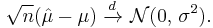
The theorem states that under certain (fairly common) conditions, the sum of a large number of random variables will have an approximately normal distribution. For example if (x1, …, xn) is a sequence of iid random variables, each having mean μ and variance σ2, then the central limit theorem states that
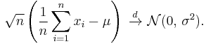
The theorem will hold even if the summands xi are not iid, although some constraints on the degree of dependence and the growth rate of moments still have to be imposed.
The importance of the central limit theorem cannot be overemphasized. A great number of test statistics, scores, and estimators encountered in practice contain sums of certain random variables in them, even more estimators can be represented as sums of random variables through the use of influence functions — all of these quantities are governed by the central limit theorem and will have asymptotically normal distribution as a result.
Another practical consequence of the central limit theorem is that certain other distributions can be approximated by the normal distribution, for example:
- The binomial distribution B(n, p) is approximately normal N(np, np(1 − p)) for large n and for p not too close to zero or one.
- The Poisson(λ) distribution is approximately normal N(λ, λ) for large values of λ.
- The chi-squared distribution χ2(k) is approximately normal N(k, 2k) for large ks.
- The Student's t-distribution t(ν) is approximately normal N(0, 1) when ν is large.
Whether these approximations are sufficiently accurate depends on the purpose for which they are needed, and the rate of convergence to the normal distribution. It is typically the case that such approximations are less accurate in the tails of the distribution.
A general upper bound for the approximation error in the central limit theorem is given by the Berry–Esseen theorem, improvements of the approximation are given by the Edgeworth expansions.
Miscellaneous
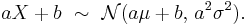
- The family of normal distributions is closed under linear transformations. That is, if X is normally distributed with mean μ and variance σ2, then a linear transform aX + b (for some real numbers a and b) is also normally distributed:
- The converse of (1) is also true: if X1 and X2 are independent and their sum X1 + X2 is distributed normally, then both X1 and X2 must also be normal.[18] This is known as Cramér's decomposition theorem. The interpretation of this property is that a normal distribution is only divisible by other normal distributions. Another application of this property is in connection with the central limit theorem: although the CLT asserts that the distribution of a sum of arbitrary non-normal iid random variables is approximately normal, the Cramér's theorem shows that it can never become exactly normal.[19]
- If the characteristic function φX of some random variable X is of the form φX(t) = eQ(t), where Q(t) is a polynomial, then the Marcinkiewicz theorem (named after Józef Marcinkiewicz) asserts that Q can be at most a quadratic polynomial, and therefore X a normal random variable.[20] The consequence of this result is that the normal distribution is the only distribution with a finite number (two) of non-zero cumulants.
- If X and Y are jointly normal and uncorrelated, then they are independent. The requirement that X and Y should be jointly normal is essential, without it the property does not hold.[proof] For non-normal random variables uncorrelatedness does not imply independence.
- If X and Y are independent N(μ, σ 2) random variables, then X + Y and X − Y are also independent and identically distributed (this follows from the polarization identity).[21] This property uniquely characterizes normal distribution, as can be seen from the Bernstein's theorem: if X and Y are independent and such that X + Y and X − Y are also independent, then both X and Y must necessarily have normal distributions.
More generally, if X1, ..., Xn are independent random variables, then two linear combinations ∑akXk and ∑bkXk will be independent if and only if all Xk's are normal and ∑akbkσ 2
k = 0, where σ 2
k denotes the variance of Xk.[22] - Normal distribution is infinitely divisible:[23] for a normally distributed X with mean μ and variance σ2 we can find n independent random variables {X1, …, Xn} each distributed normally with means μ/n and variances σ2/n such that
- Normal distribution is stable (with exponent α = 2): if X1, X2 are two independent N(μ, σ2) random variables and a, b are arbitrary real numbers, then
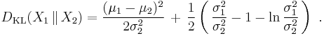
- The Kullback–Leibler divergence between two normal distributions X1 ∼ N(μ1, σ21 )and X2 ∼ N(μ2, σ22 )is given by:[24]
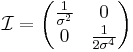
- The Fisher information matrix for normal distribution is diagonal and takes form
- Normal distributions belongs to an exponential family with natural parameters
 and
and  , and natural statistics x and x2. The dual, expectation parameters for normal distribution are η1 = μ and η2 = μ2 + σ2.
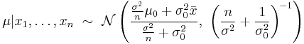
 - The conjugate prior of the mean of a normal distribution is another normal distribution.[25] Specifically, if x1, …, xn are iid N(μ, σ2) and the prior is μ ~ N(μ0, σ2
0), then the posterior distribution for the estimator of μ will be - Of all probability distributions over the reals with mean μ and variance σ2, the normal distribution N(μ, σ2) is the one with the maximum entropy.[26]
- The family of normal distributions forms a manifold with constant curvature −1. The same family is flat with respect to the (±1)-connections ∇(e) and ∇(m).[27]


Related distributions
Operations on a single random variable
If X is distributed normally with mean μ and variance σ2, then
- The exponential of X is distributed log-normally: eX ~ lnN (μ, σ2).
- The absolute value of X has folded normal distribution: IXI ~ Nf (μ, σ2). If μ = 0 this is known as the half-normal distribution.
- The square of X/σ has the noncentral chi-squared distribution with one degree of freedom: X2/σ2 ~ χ21(μ2/σ2). If μ = 0, the distribution is called simply chi-squared.
- The distribution of the variable X restricted to an interval [a, b] is called the truncated normal distribution.
- (X − μ)−2 has a Lévy distribution with location 0 and scale σ−2.
Combination of two independent random variables
If X1 and X2 are two independent standard normal random variables, then
- Their sum and difference is distributed normally with mean zero and variance two: X1 ± X2 ∼ N(0, 2).
- Their product Z = X1·X2 follows the "product-normal" distribution[28] with density function fZ(z) = π−1K0(|z|), where K0 is the modified Bessel function of the second kind. This distribution is symmetric around zero, unbounded at z = 0, and has the characteristic function φZ(t) = (1 + t 2)−1/2.
- Their ratio follows the standard Cauchy distribution: X1 ÷ X2 ∼ Cauchy(0, 1).
- Their Euclidean norm
 has the Rayleigh distribution, also known as the chi distribution with 2 degrees of freedom.
Combination of two or more independent random variables
- If X1, X2, …, Xn are independent standard normal random variables, then the sum of their squares has the chi-squared distribution with n degrees of freedom:
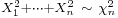 .
. - If X1, X2, …, Xn are independent normally distributed random variables with means μ and variances σ2, then their sample mean is independent from the sample standard deviation, which can be demonstrated using the Basu's theorem or Cochran's theorem. The ratio of these two quantities will have the Student's t-distribution with n − 1 degrees of freedom:
![t = \frac{\overline X - \mu}{S/\sqrt{n}} = \frac{\frac{1}{n}(X_1%2B\cdots%2BX_n) - \mu}{\sqrt{\frac{1}{n(n-1)}\left[(X_1-\overline X)^2%2B\cdots%2B(X_n-\overline X)^2\right]}} \ \sim\ t_{n-1}.](/2012-wikipedia_en_all_nopic_01_2012/I/35addf92e4d247fe1e2436780514b88e.png)
- If X1, …, Xn, Y1, …, Ym are independent standard normal random variables, then the ratio of their normalized sums of squares will have the F-distribution with (n, m) degrees of freedom:
Operations on the density function
The split normal distribution is most directly defined in terms of joining scaled sections of the density functions of different normal distributions and rescaling the density to integrate to one. The truncated normal distribution results from rescaling a section of a single density function.
Extensions
The notion of normal distribution, being one of the most important distributions in probability theory, has been extended far beyond the standard framework of the univariate (that is one-dimensional) case (Case 1). All these extensions are also called normal or Gaussian laws, so a certain ambiguity in names exists.
- Multivariate normal distribution describes the Gaussian law in the k-dimensional Euclidean space. A vector X ∈ Rk is multivariate-normally distributed if any linear combination of its components ∑k
j=1aj Xj has a (univariate) normal distribution. The variance of X is a k×k symmetric positive-definite matrix V. - Rectified Gaussian distribution a rectified version of normal distribution with all the negative elements reset to 0
- Complex normal distribution deals with the complex normal vectors. A complex vector X ∈ Ck is said to be normal if both its real and imaginary components jointly possess a 2k-dimensional multivariate normal distribution. The variance-covariance structure of X is described by two matrices: the variance matrix Γ, and the relation matrix C.
- Matrix normal distribution describes the case of normally distributed matrices.
- Gaussian processes are the normally distributed stochastic processes. These can be viewed as elements of some infinite-dimensional Hilbert space H, and thus are the analogues of multivariate normal vectors for the case k = ∞. A random element h ∈ H is said to be normal if for any constant a ∈ H the scalar product (a, h) has a (univariate) normal distribution. The variance structure of such Gaussian random element can be described in terms of the linear covariance operator K: H → H. Several Gaussian processes became popular enough to have their own names:
- Gaussian q-distribution is an abstract mathematical construction which represents a "q-analogue" of the normal distribution.
- the q-Gaussian is an analogue of the Gaussian distribution, in the sense that it maximises the Tsallis entropy, and is one type of Tsallis distribution. Note that this distribution is different from the Gaussian q-distribution above.
One of the main practical uses of the Gaussian law is to model the empirical distributions of many different random variables encountered in practice. In such case a possible extension would be a richer family of distributions, having more than two parameters and therefore being able to fit the empirical distribution more accurately. The examples of such extensions are:
- Pearson distribution — a four-parametric family of probability distributions that extend the normal law to include different skewness and kurtosis values.
Normality tests
Normality tests assess the likelihood that the given data set {x1, …, xn} comes from a normal distribution. Typically the null hypothesis H0 is that the observations are distributed normally with unspecified mean μ and variance σ2, versus the alternative Ha that the distribution is arbitrary. A great number of tests (over 40) have been devised for this problem, the more prominent of them are outlined below:
- "Visual" tests are more intuitively appealing but subjective at the same time, as they rely on informal human judgement to accept or reject the null hypothesis.
- Q-Q plot — is a plot of the sorted values from the data set against the expected values of the corresponding quantiles from the standard normal distribution. That is, it's a plot of point of the form (Φ−1(pk), x(k)), where plotting points pk are equal to pk = (k − α)/(n + 1 − 2α) and α is an adjustment constant which can be anything between 0 and 1. If the null hypothesis is true, the plotted points should approximately lie on a straight line.
- P-P plot — similar to the Q-Q plot, but used much less frequently. This method consists of plotting the points (Φ(z(k)), pk), where
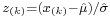 . For normally distributed data this plot should lie on a 45° line between (0, 0) and (1, 1).
 - Wilk–Shapiro test employs the fact that the line in the Q-Q plot has the slope of σ. The test compares the least squares estimate of that slope with the value of the sample variance, and rejects the null hypothesis if these two quantities differ significantly.
- Normal probability plot (rankit plot)
- Moment tests:
- Empirical distribution function tests:
- Lilliefors test (an adaptation of the Kolmogorov–Smirnov test)
- Anderson–Darling test
Estimation of parameters
It is often the case that we don't know the parameters of the normal distribution, but instead want to estimate them. That is, having a sample (x1, …, xn) from a normal N(μ, σ2) population we would like to learn the approximate values of parameters μ and σ2. The standard approach to this problem is the maximum likelihood method, which requires maximization of the log-likelihood function:

Taking derivatives with respect to μ and σ2 and solving the resulting system of first order conditions yields the maximum likelihood estimates:
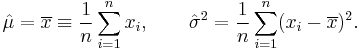
Estimator  is called the sample mean, since it is the arithmetic mean of all observations. The statistic
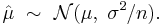
  is complete and sufficient for μ, and therefore by the Lehmann–Scheffé theorem, is the uniformly minimum variance unbiased (UMVU) estimator.[29] In finite samples it is distributed normally:
The variance of this estimator is equal to the μμ-element of the inverse Fisher information matrix  . This implies that the estimator is finite-sample efficient. Of practical importance is the fact that the standard error of is proportional to
  , that is, if one wishes to decrease the standard error by a factor of 10, one must increase the number of points in the sample by a factor of 100. This fact is widely used in determining sample sizes for opinion polls and the number of trials in Monte Carlo simulations.
From the standpoint of the asymptotic theory, is consistent, that is, it converges in probability to μ as n → ∞. The estimator is also asymptotically normal, which is a simple corollary of the fact that it is normal in finite samples:
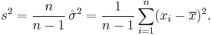
The estimator  is called the sample variance, since it is the variance of the sample (x1, …, xn). In practice, another estimator is often used instead of the . This other estimator is denoted s2, and is also called the sample variance, which represents a certain ambiguity in terminology; its square root s is called the sample standard deviation. The estimator s2 differs from by having (n − 1) instead of n in the denominator (the so called Bessel's correction):
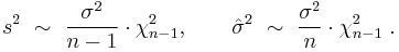
The difference between s2 and becomes negligibly small for large n's. In finite samples however, the motivation behind the use of s2 is that it is an unbiased estimator of the underlying parameter σ2, whereas is biased. Also, by the Lehmann–Scheffé theorem the estimator s2 is uniformly minimum variance unbiased (UMVU),[29] which makes it the "best" estimator among all unbiased ones. However it can be shown that the biased estimator is "better" than the s2 in terms of the mean squared error (MSE) criterion. In finite samples both s2 and have scaled chi-squared distribution with (n − 1) degrees of freedom:
The first of these expressions shows that the variance of s2 is equal to 2σ4/(n−1), which is slightly greater than the σσ-element of the inverse Fisher information matrix . Thus, s2 is not an efficient estimator for σ2, and moreover, since s2 is UMVU, we can conclude that the finite-sample efficient estimator for σ2 does not exist.
Applying the asymptotic theory, both estimators s2 and are consistent, that is they converge in probability to σ2 as the sample size n → ∞. The two estimators are also both asymptotically normal:

In particular, both estimators are asymptotically efficient for σ2.
By Cochran's theorem, for normal distribution the sample mean and the sample variance s2 are independent, which means there can be no gain in considering their joint distribution. There is also a reverse theorem: if in a sample the sample mean and sample variance are independent, then the sample must have come from the normal distribution. The independence between and s can be employed to construct the so-called t-statistic:
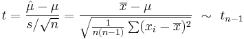
This quantity t has the Student's t-distribution with (n − 1) degrees of freedom, and it is an ancillary statistic (independent of the value of the parameters). Inverting the distribution of this t-statistics will allow us to construct the confidence interval for μ;[30] similarly, inverting the χ2 distribution of the statistic s2 will give us the confidence interval for σ2:[31]
![\begin{align}
& \mu \in \left[\, \hat\mu %2B t_{n-1,\alpha/2}\, \frac{1}{\sqrt{n}}s,\ \
\hat\mu %2B t_{n-1,1-\alpha/2}\,\frac{1}{\sqrt{n}}s \,\right] \approx
\left[\, \hat\mu - |z_{\alpha/2}|\frac{1}{\sqrt n}s,\ \
\hat\mu %2B |z_{\alpha/2}|\frac{1}{\sqrt n}s \,\right], \\
& \sigma^2 \in \left[\, \frac{(n-1)s^2}{\chi^2_{n-1,1-\alpha/2}},\ \
\frac{(n-1)s^2}{\chi^2_{n-1,\alpha/2}} \,\right] \approx
\left[\, s^2 - |z_{\alpha/2}|\frac{\sqrt{2}}{\sqrt{n}}s^2,\ \
s^2 %2B |z_{\alpha/2}|\frac{\sqrt{2}}{\sqrt{n}}s^2 \,\right],
\end{align}](/2012-wikipedia_en_all_nopic_01_2012/I/a3d966d4dfadbaa6e1d74e21716cb4b9.png)
where tk,p and χ 2
k,p are the pth quantiles of the t- and χ2-distributions respectively. These confidence intervals are of the level 1 − α, meaning that the true values μ and σ2 fall outside of these intervals with probability α. In practice people usually take α = 5%, resulting in the 95% confidence intervals. The approximate formulas in the display above were derived from the asymptotic distributions of and s2. The approximate formulas become valid for large values of n, and are more convenient for the manual calculation since the standard normal quantiles zα/2 do not depend on n. In particular, the most popular value of α = 5%, results in |z0.025| = 1.96.
Occurrence
The occurrence of normal distribution in practical problems can be loosely classified into three categories:
- Exactly normal distributions;
- Approximately normal laws, for example when such approximation is justified by the central limit theorem; and
- Distributions modeled as normal — the normal distribution being the distribution with maximum entropy for a given mean and variance.
Exact normality
Certain quantities in physics are distributed normally, as was first demonstrated by James Clerk Maxwell. Examples of such quantities are:
- Velocities of the molecules in the ideal gas. More generally, velocities of the particles in any system in thermodynamic equilibrium will have normal distribution, due to the maximum entropy principle.
- Probability density function of a ground state in a quantum harmonic oscillator.
- The position of a particle which experiences diffusion. If initially the particle is located at a specific point (that is its probability distribution is the dirac delta function), then after time t its location is described by a normal distribution with variance t, which satisfies the diffusion equation ∂∂t f(x,t) = 12 ∂2∂x2 f(x,t). If the initial location is given by a certain density function g(x), then the density at time t is the convolution of g and the normal PDF.
Approximate normality
Approximately normal distributions occur in many situations, as explained by the central limit theorem. When the outcome is produced by a large number of small effects acting additively and independently, its distribution will be close to normal. The normal approximation will not be valid if the effects act multiplicatively (instead of additively), or if there is a single external influence which has a considerably larger magnitude than the rest of the effects.
- In counting problems, where the central limit theorem includes a discrete-to-continuum approximation and where infinitely divisible and decomposable distributions are involved, such as
- Binomial random variables, associated with binary response variables;
- Poisson random variables, associated with rare events;
- Thermal light has a Bose–Einstein distribution on very short time scales, and a normal distribution on longer timescales due to the central limit theorem.
Assumed normality
| “ | I can only recognize the occurrence of the normal curve — the Laplacian curve of errors — as a very abnormal phenomenon. It is roughly approximated to in certain distributions; for this reason, and on account for its beautiful simplicity, we may, perhaps, use it as a first approximation, particularly in theoretical investigations. — Pearson (1901) | ” |
There are statistical methods to empirically test that assumption, see the above Normality tests section.
- In biology, the logarithm of various variables tend to have a normal distribution, that is, they tend to have a log-normal distribution (after separation on male/female subpopulations), with examples including:
- Measures of size of living tissue (length, height, skin area, weight);[32]
- The length of inert appendages (hair, claws, nails, teeth) of biological specimens, in the direction of growth; presumably the thickness of tree bark also falls under this category;
- Certain physiological measurements, such as blood pressure of adult humans.
- In finance, in particular the Black–Scholes model, changes in the logarithm of exchange rates, price indices, and stock market indices are assumed normal (these variables behave like compound interest, not like simple interest, and so are multiplicative). Some mathematicians such as Benoît Mandelbrot have argued that log-Levy distributions which possesses heavy tails would be a more appropriate model, in particular for the analysis for stock market crashes.
- Measurement errors in physical experiments are often modeled by a normal distribution. This use of a normal distribution does not imply that one is assuming the measurement errors are normally distributed, rather using the normal distribution produces the most conservative predictions possible given only knowledge about the mean and variance of the errors.[33]
- In standardized testing, results can be made to have a normal distribution. This is done by either selecting the number and difficulty of questions (as in the IQ test), or by transforming the raw test scores into "output" scores by fitting them to the normal distribution. For example, the SAT's traditional range of 200–800 is based on a normal distribution with a mean of 500 and a standard deviation of 100.
- Many scores are derived from the normal distribution, including percentile ranks ("percentiles" or "quantiles"), normal curve equivalents, stanines, z-scores, and T-scores. Additionally, a number of behavioral statistical procedures are based on the assumption that scores are normally distributed; for example, t-tests and ANOVAs. Bell curve grading assigns relative grades based on a normal distribution of scores.
- In hydrology the distribution of long duration river discharge or rainfall (e.g. monthly and yearly totals, consisting of the sum of 30 respectively 360 daily values) is often thought to be practically normal according to the central limit theorem.[34] The blue picture illustrates an example of fitting the normal distribution to ranked October rainfalls showing the 90% confidence belt based on the binomial distribution. The rainfall data are represented by plotting positions as part of the cumulative frequency analysis.
Generating values from normal distribution
In computer simulations, especially in applications of the Monte-Carlo method, it is often desirable to generate values that are normally distributed. The algorithms listed below all generate the standard normal deviates, since a N(μ, σ2
) can be generated as X = μ + σZ, where Z is standard normal. All these algorithms rely on the availability of a random number generator U capable of producing uniform random variates.
- The most straightforward method is based on the probability integral transform property: if U is distributed uniformly on (0,1), then Φ−1(U) will have the standard normal distribution. The drawback of this method is that it relies on calculation of the probit function Φ−1, which cannot be done analytically. Some approximate methods are described in Hart (1968) and in the erf article.
- An easy to program approximate approach, that relies on the central limit theorem, is as follows: generate 12 uniform U(0,1) deviates, add them all up, and subtract 6 — the resulting random variable will have approximately standard normal distribution. In truth, the distribution will be Irwin–Hall, which is a 12-section eleventh-order polynomial approximation to the normal distribution. This random deviate will have a limited range of (−6, 6).[35]
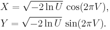
- The Box–Muller method uses two independent random numbers U and V distributed uniformly on (0,1). Then the two random variables X and Y
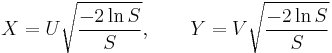
- Marsaglia polar method is a modification of the Box–Muller method algorithm, which does not require computation of functions sin() and cos(). In this method U and V are drawn from the uniform (−1,1) distribution, and then S = U2 + V2 is computed. If S is greater or equal to one then the method starts over, otherwise two quantities
- The Ratio method[36] is a rejection method. The algorithm proceeds as follows:
- Generate two independent uniform deviates U and V;
- Compute X = √8/e (V − 0.5)/U;
- If X2 ≤ 5 − 4e1/4U then accept X and terminate algorithm;
- If X2 ≥ 4e−1.35/U + 1.4 then reject X and start over from step 1;
- If X2 ≤ −4 / lnU then accept X, otherwise start over the algorithm.
- The ziggurat algorithm (Marsaglia & Tsang 2000) is faster than the Box–Muller transform and still exact. In about 97% of all cases it uses only two random numbers, one random integer and one random uniform, one multiplication and an if-test. Only in 3% of the cases where the combination of those two falls outside the "core of the ziggurat" a kind of rejection sampling using logarithms, exponentials and more uniform random numbers has to be employed.
- There is also some investigation into the connection between the fast Hadamard transform and the normal distribution, since the transform employs just addition and subtraction and by the central limit theorem random numbers from almost any distribution will be transformed into the normal distribution. In this regard a series of Hadamard transforms can be combined with random permutations to turn arbitrary data sets into a normally distributed data.
Numerical approximations for the normal CDF
The standard normal CDF is widely used in scientific and statistical computing. The values Φ(x) may be approximated very accurately by a variety of methods, such as numerical integration, Taylor series, asymptotic series and continued fractions. Different approximations are used depending on the desired level of accuracy.
- Abramowitz & Stegun (1964) give the approximation for Φ(x) for x > 0 with the absolute error |ε(x)| < 7.5·10−8 (algorithm 26.2.17):
- Hart (1968) lists almost a hundred of rational function approximations for the erfc() function. His algorithms vary in the degree of complexity and the resulting precision, with maximum absolute precision of 24 digits. An algorithm by West (2009) combines Hart's algorithm 5666 with a continued fraction approximation in the tail to provide a fast computation algorithm with a 16-digit precision.
- W. J. Cody (1969) after recalling Hart68 solution is not suited for erf, gives a solution for both erf and erfc, with maximal relative error bound, via Rational Chebyshev Approximation. (Cody, W. J. (1969). "Rational Chebyshev Approximations for the Error Function", paper here).
- Marsaglia (2004) suggested a simple algorithm[nb 2] based on the Taylor series expansion
- The GNU Scientific Library calculates values of the standard normal CDF using Hart's algorithms and approximations with Chebyshev polynomials.


History
Development
Some authors[37][38] attribute the credit for the discovery of the normal distribution to de Moivre, who in 1738 [nb 3] published in the second edition of his "The Doctrine of Chances" the study of the coefficients in the binomial expansion of (a + b)n. De Moivre proved that the middle term in this expansion has the approximate magnitude of  , and that "If m or ½n be a Quantity infinitely great, then the Logarithm of the Ratio, which a Term distant from the middle by the Interval ℓ, has to the middle Term, is
  ."[39] Although this theorem can be interpreted as the first obscure expression for the normal probability law, Stigler points out that de Moivre himself did not interpret his results as anything more than the approximate rule for the binomial coefficients, and in particular de Moivre lacked the concept of the probability density function.[40]
In 1809 Gauss published his monograph "Theoria motus corporum coelestium in sectionibus conicis solem ambientium" where among other things he introduces several important statistical concepts, such as the method of least squares, the method of maximum likelihood, and the normal distribution. Gauss used M, M′, M′′, … to denote the measurements of some unknown quantity V, and sought the "most probable" estimator: the one which maximizes the probability φ(M−V) · φ(M′−V) · φ(M′′−V) · … of obtaining the observed experimental results. In his notation φΔ is the probability law of the measurement errors of magnitude Δ. Not knowing what the function φ is, Gauss requires that his method should reduce to the well-known answer: the arithmetic mean of the measured values.[nb 4] Starting from these principles, Gauss demonstrates that the only law which rationalizes the choice of arithmetic mean as an estimator of the location parameter, is the normal law of errors:[41]
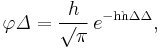
where h is "the measure of the precision of the observations". Using this normal law as a generic model for errors in the experiments, Gauss formulates what is now known as the non-linear weighted least squares (NWLS) method.[42]
Although Gauss was the first to suggest the normal distribution law, Laplace made significant contributions.[nb 5] It was Laplace who first posed the problem of aggregating several observations in 1774,[43] although his own solution led to the Laplacian distribution. It was Laplace who first calculated the value of the integral ∫ e−t ²dt = √π in 1782, providing the normalization constant for the normal distribution.[44] Finally, it was Laplace who in 1810 proved and presented to the Academy the fundamental central limit theorem, which emphasized the theoretical importance of the normal distribution.[45]
It is of interest to note that in 1809 an American mathematician Adrain published two derivations of the normal probability law, simultaneously and independently from Gauss.[46] His works remained largely unnoticed by the scientific community, until in 1871 they were "rediscovered" by Abbe.[47]
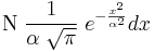
In the middle of the 19th century Maxwell demonstrated that the normal distribution is not just a convenient mathematical tool, but may also occur in natural phenomena:[48] "The number of particles whose velocity, resolved in a certain direction, lies between x and x + dx is
Naming
Since its introduction, the normal distribution has been known by many different names: the law of error, the law of facility of errors, Laplace's second law, Gaussian law, etc. By the end of the 19th century some authors[nb 6] had started using the name normal distribution, where the word "normal" was used as an adjective — the term was derived from the fact that this distribution was seen as typical, common, normal. Peirce (one of those authors) once defined "normal" thus: "...the 'normal' is not the average (or any other kind of mean) of what actually occurs, but of what would, in the long run, occur under certain circumstances."[49] Around the turn of the 20th century Pearson popularized the term normal as a designation for this distribution.[50]
| “ | Many years ago I called the Laplace–Gaussian curve the normal curve, which name, while it avoids an international question of priority, has the disadvantage of leading people to believe that all other distributions of frequency are in one sense or another 'abnormal'. — Pearson (1920) | ” |
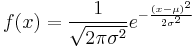
Also, it was Pearson who first wrote the distribution in terms of the standard deviation σ as in modern notation. Soon after this, in year 1915, Fisher added the location parameter to the formula for normal distribution, expressing it in the way it is written nowadays:
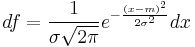
The term "standard normal" which denotes the normal distribution with zero mean and unit variance came into general use around 1950s, appearing in the popular textbooks by P.G. Hoel (1947) "Introduction to mathematical statistics" and A.M. Mood (1950) "Introduction to the theory of statistics".[51]
When the name is used, the "Gaussian distribution" was named after Carl Friedrich Gauss, who introduced the distribution in 1809 as a way of rationalizing the method of least squares as outlined above. The related work of Laplace, also outlined above has led to the normal distribution being sometimes called Laplacian, especially in French-speaking countries. Among English speakers, both "normal distribution" and "Gaussian distribution" are in common use, with different terms preferred by different communities.
See also
- Behrens–Fisher problem—the long-standing problem of testing whether two normal samples with different variances have same means;
- Erdős–Kac theorem—on the occurrence of the normal distribution in number theory
- Gaussian blur—convolution which uses the normal distribution as a kernel
- Sum of normally distributed random variables
Notes
- ^ The designation "bell curve" is ambiguous: there are many other distributions which are "bell"-shaped: the Cauchy distribution, Student's t-distribution, generalized normal, logistic, etc.
- ^ For example, this algorithm is given in the article Bc programming language.
- ^ De Moivre first published his findings in 1733, in a pamphlet "Approximatio ad Summam Terminorum Binomii (a + b)n in Seriem Expansi" that was designated for private circulation only. But it was not until the year 1738 that he made his results publicly available. The original pamphlet was reprinted several times, see for example Walker (1985).
- ^ "It has been customary certainly to regard as an axiom the hypothesis that if any quantity has been determined by several direct observations, made under the same circumstances and with equal care, the arithmetical mean of the observed values affords the most probable value, if not rigorously, yet very nearly at least, so that it is always most safe to adhere to it." — Gauss (1809, section 177)
- ^ "My custom of terming the curve the Gauss–Laplacian or normal curve saves us from proportioning the merit of discovery between the two great astronomer mathematicians." quote from Pearson (1905, p. 189)
- ^ Besides those specifically referenced here, such use is encountered in the works of Peirce, Galton and Lexis approximately around 1875.
Citations
- ^ Casella & Berger (2001, p. 102)
- ^ Gale Encyclopedia of Psychology — Normal Distribution
- ^ Cover, T. M.; Thomas, Joy A (2006). Elements of information theory. John Wiley and Sons. p. 254.
- ^ Park, Sung Y.; Bera, Anil K. (2009). "Maximum entropy autoregressive conditional heteroskedasticity model". Journal of Econometrics (Elsevier): 219–230. http://www.wise.xmu.edu.cn/Master/Download/..%5C..%5CUploadFiles%5Cpaper-masterdownload%5C2009519932327055475115776.pdf. Retrieved 2011-06-02.
- ^ Halperin & et al. (1965, item 7)
- ^ McPherson (1990, p. 110)
- ^ Bernardo & Smith (2000)
- ^ a b c Patel & Read (1996, [2.1.4])
- ^ Fan (1991, p. 1258)
- ^ Patel & Read (1996, [2.1.8])
- ^ Scott, Clayton; Robert Nowak (August 7, 2003). "The Q-function". Connexions. http://cnx.org/content/m11537/1.2/.
- ^ Barak, Ohad (April 6, 2006). "Q function and error function". Tel Aviv University. http://www.eng.tau.ac.il/~jo/academic/Q.pdf.
- ^ Weisstein, Eric W., "Normal Distribution Function" from MathWorld.
- ^ Bryc (1995, p. 23)
- ^ Bryc (1995, p. 24)
- ^ WolframAlpha.com
- ^ part 1, part 2
- ^ Galambos & Simonelli (2004, Theorem 3.5)
- ^ Bryc (2995, p. 35)
- ^ Bryc (1995, p. 35)
- ^ Bryc (1995, p. 27)
- ^ Lukacs & King (1954)
- ^ Patel & Read (1996, [2.3.6])
- ^ http://www.allisons.org/ll/MML/KL/Normal/
- ^ "Stat260: Bayesian Modeling and Inference Lecture Date: February 8th, 2010, The Conjugate Prior for the Normal Distribution, Lecturer: Michael I. Jordan|". http://www.cs.berkeley.edu/~jordan/courses/260-spring10/lectures/lecture5.pdf.
- ^ Cover & Thomas (2006, p. 254)
- ^ Amari & Nagaoka (2000)
- ^ Mathworld entry for Normal Product Distribution
- ^ a b Krishnamoorthy (2006, p. 127)
- ^ Krishnamoorthy (2006, p. 130)
- ^ Krishnamoorthy (2006, p. 133)
- ^ Huxley (1932)
- ^ Jaynes, E. T. (2003). Probability Theory: The Logic of Science. Cambridge University Press. pp. 592–593.
- ^ Ritzema (ed.), H.P. (1994). Frequency and Regression Analysis. Chapter 6 in: Drainage Principles and Applications, Publication 16, International Institute for Land Reclamation and Improvement (ILRI), Wageningen, The Netherlands. pp. 175–224. ISBN 90 70754 3 39. http://www.waterlog.info/pdf/freqtxt.pdf.
- ^ Johnson et al. (1995, Equation (26.48))
- ^ Kinderman & Monahan (1976)
- ^ Johnson et al. (1994, page 85)
- ^ Le Cam (2000, p. 74)
- ^ De Moivre (1733), Corollary I — see Walker (1985, p. 77)
- ^ Stigler (1986, p. 76)
- ^ Gauss (1809, section 177)
- ^ Gauss (1809, section 179)
- ^ Laplace (1774, Problem III)
- ^ Pearson (1905, p. 189)
- ^ Stigler (1986, p. 144)
- ^ Stigler (1978, p. 243)
- ^ Stigler (1978, p. 244)
- ^ Maxwell (1860), p. 23
- ^ Peirce, C. S. (c. 1909 MS), Collected Papers v. 6, paragraph 327.
- ^ Kruskal & Stigler (1997)
- ^ "Earliest uses… (entry STANDARD NORMAL CURVE)". http://jeff560.tripod.com/s.html.
References
- Aldrich, John; Miller, Jeff. "Earliest uses of symbols in probability and statistics". http://jeff560.tripod.com/stat.html.
- Aldrich, John; Miller, Jeff. "Earliest known uses of some of the words of mathematics". http://jeff560.tripod.com/mathword.html. In particular, the entries for "bell-shaped and bell curve", "normal (distribution)", "Gaussian", and "Error, law of error, theory of errors, etc.".
- Amari, Shun-ichi; Nagaoka, Hiroshi (2000). Methods of information geometry. Oxford University Press. ISBN 0-8218-0531-2.
- Bernardo, J. M.; Smith, A.F.M. (2000). Bayesian Theory. Wiley. ISBN 0-471-49464-X.
- Bryc, Wlodzimierz (1995). The normal distribution: characterizations with applications. Springer-Verlag. ISBN 0-387-97990-5.
- Casella, George; Berger, Roger L. (2001). Statistical inference (2nd ed.). Duxbury. ISBN 0-534-24312-6.
- Cover, T. M.; Thomas, Joy A. (2006). Elements of information theory. John Wiley and Sons.
- de Moivre, Abraham (1738). The Doctrine of Chances. ISBN 0821821032.
- Fan, Jianqing (1991). "On the optimal rates of convergence for nonparametric deconvolution problems". The Annals of Statistics 19 (3): 1257–1272. doi:10.1214/aos/1176348248. JSTOR 2241949.
- Galambos, Janos; Simonelli, Italo (2004). Products of random variables: applications to problems of physics and to arithmetical functions. Marcel Dekker, Inc.. ISBN 0-8247-5402-6.
- Gauss, Carolo Friderico (1809) (in Latin). Theoria motvs corporvm coelestivm in sectionibvs conicis Solem ambientivm [Theory of the motion of the heavenly bodies moving about the Sun in conic sections]. English translation.
- Gould, Stephen Jay (1981). The mismeasure of man (first ed.). W.W. Norton. ISBN 0-393-01489-4.
- Halperin, Max; Hartley, H. O.; Hoel, P. G. (1965). "Recommended standards for statistical symbols and notation. COPSS committee on symbols and notation". The American Statistician 19 (3): 12–14. doi:10.2307/2681417. JSTOR 2681417.
- Hart, John F.; et al (1968). Computer approximations. New York: John Wiley & Sons, Inc. ISBN 0882756427.
- Herrnstein, C.; Murray (1994). The bell curve: intelligence and class structure in American life. Free Press. ISBN 0-02-914673-9.
- Huxley, Julian S. (1932). Problems of relative growth. London. ISBN 0486611140. OCLC 476909537.
- Johnson, N.L.; Kotz, S.; Balakrishnan, N. (1994). Continuous univariate distributions, Volume 1. Wiley. ISBN 0-471-58495-9.
- Johnson, N.L.; Kotz, S.; Balakrishnan, N. (1995). Continuous univariate distributions, Volume 2. Wiley. ISBN 0-471-58494-0.
- Krishnamoorthy, K. (2006). Handbook of statistical distributions with applications. Chapman & Hall/CRC. ISBN 1-58488-635-8.
- Kruskal, William H.; Stigler, Stephen M. (1997). Normative terminology: 'normal' in statistics and elsewhere. Statistics and public policy, edited by Bruce D. Spencer. Oxford University Press. ISBN 0-19-852341-6.
- la Place, M. de (1774). "Mémoire sur la probabilité des causes par les évènemens". Mémoires de Mathématique et de Physique, Presentés à l'Académie Royale des Sciences, par divers Savans & lûs dans ses Assemblées, Tome Sixième: 621–656. Translated by S.M.Stigler in Statistical Science 1 (3), 1986: JSTOR 2245476.
- Laplace, Pierre-Simon (1812). Analytical theory of probabilities.
- Lukacs, Eugene; King, Edgar P. (1954). "A property of normal distribution". The Annals of Mathematical Statistics 25 (2): 389–394. doi:10.1214/aoms/1177728796. JSTOR 2236741.
- McPherson, G. (1990). Statistics in scientific investigation: its basis, application and interpretation. Springer-Verlag. ISBN 0-387-97137-8.
- Marsaglia, George; Tsang, Wai Wan (2000). "The ziggurat method for generating random variables". Journal of Statistical Software 5 (8). http://www.jstatsoft.org/v05/i08/paper.
- Marsaglia, George (2004). "Evaluating the normal distribution". Journal of Statistical Software 11 (4). http://www.jstatsoft.org/v11/i05/paper.
- Maxwell, James Clerk (1860). "V. Illustrations of the dynamical theory of gases. — Part I: On the motions and collisions of perfectly elastic spheres". Philosophical Magazine, series 4 19 (124): 19–32. doi:10.1080/14786446008642818.
- Patel, Jagdish K.; Read, Campbell B. (1996). Handbook of the normal distribution (2nd ed.). CRC Press. ISBN 0-824-79342-0.
- Pearson, Karl (1905). "'Das Fehlergesetz und seine Verallgemeinerungen durch Fechner und Pearson'. A rejoinder". Biometrika 4 (1): 169–212. JSTOR 2331536.
- Pearson, Karl (1920). "Notes on the history of correlation". Biometrika 13 (1): 25–45. doi:10.1093/biomet/13.1.25. JSTOR 2331722.
- Stigler, Stephen M. (1978). "Mathematical statistics in the early states". The Annals of Statistics 6 (2): 239–265. doi:10.1214/aos/1176344123. JSTOR 2958876.
- Stigler, Stephen M. (1982). "A modest proposal: a new standard for the normal". The American Statistician 36 (2): 137–138. doi:10.2307/2684031. JSTOR 2684031.
- Stigler, Stephen M. (1986). The history of statistics: the measurement of uncertainty before 1900. Harvard University Press. ISBN 0-674-40340-1.
- Stigler, Stephen M. (1999). Statistics on the table. Harvard University Press. ISBN 0674836014.
- Walker, Helen M (1985). "De Moivre on the law of normal probability". In Smith, David Eugene. A source book in mathematics. Dover. ISBN 0486646904. http://www.york.ac.uk/depts/maths/histstat/demoivre.pdf.
- Weisstein, Eric W. "Normal distribution". MathWorld. http://mathworld.wolfram.com/NormalDistribution.html.
- West, Graeme (2009). "Better approximations to cumulative normal functions". Wilmott Magazine: 70–76. http://www.wilmott.com/pdfs/090721_west.pdf.
- Zelen, Marvin; Severo, Norman C. (1964). Probability functions (chapter 26). Handbook of mathematical functions with formulas, graphs, and mathematical tables, by Abramowitz and Stegun: National Bureau of Standards. New York: Dover. ISBN 0-486-61272-4. http://www.math.sfu.ca/~cbm/aands/page_931.htm.
External links
- Normal Distribution Video Tutorial Part 1-2
- An 8-foot-tall (2.4 m) Probability Machine (named Sir Francis) comparing stock market returns to the randomness of the beans dropping through the quincunx pattern. YouTube link originating from Index Funds Advisors
|
|||||||||||